Particles

In this tutorial we will show how to add particles to a BHAC simulation. Particles can be used to track the motion of fluid elements and to register properties of the fluid, or ‘payloads’, along the particle’s path. Depending on the particle pusher chosen, this can be the worldine of a fluid element (or a streamline if the background simulation is not evolving), a charged particle, or the geodesic of a massive or massless particle.

We will work with the setup ‘FMTorus’, that can be found in $BHAC_DIR/tests/rmhd/FMtorus

Adding particles to a simulation

Copy the folder containing the set-up to a working directory.

cp -r $BHAC_DIR/tests/rmhd/FMtorus ./
cd FMtorus

To add particles to the simulation, edit the file definitions.h and add

# define PARTICLES_ADVECT

This will add particles that are advected with the fluid velocity. There are also other possibilities, here there is a complete list:

PARTICLES_ADVECT : Advects particles with the fluid velocity
PARTICLES_LORENTZ : Pushes particles with the Lorentz force (only for Cartesian coordinates)
PARTICLES_GEODESIC : Pushes particles along geodesics
PARTICLES_GRLORENTZ : Pushes particles with the Lorentz force on a curved spacetime

After editing defininitions.t,

make

and create the output directory

mkdir output

Now, to run a simulation with particles, we need to edit also the parameter file, in this case amrvac.par

Inside the &methodlist, add

   use_particles = .true.

And add the following list to the file:

&particleslist
    nparticleshi = 10000
    nparticles_per_cpu_hi = 1000
    nparticles_init = 1000
    npayload = 0
    write_ensemble = .true.
    dtsave_ensemble = 1.0d0
    ensemble_type = 'csv'
    write_individual = .false.
    dtsave_individual = 0.1d0
&end

The &particlelist contains parameters such as the number of particles to be initialized (nparticles_init), the maximum number of particles allowed in the simulation (nparticleshi) or per CPU (nparticles_per_cpu_high). Other important parameters are the times to save and the kind of output files.

We can now run our first simulation with particles using e.g.

mpiexec -n 4 ./bhac

When running, we will notice that the simulations now outputs to the screen messages that indicate when a particle has left from the simulation (all particles will show this message at the end of the
simulation).

We will also notice that the output directory now contains different kind of files related to particles, such as:

data_particles0000.dat
data0000_ensemble000000.csv
data0000_particle000001.csv

Reading particle files.

The particle output files contain different kinds of information. The ‘ensemble’ files contain a snapshot of the positions and velocities of all the particles at a given step, while the ‘particle’ files contain information on the history of a given individual particle. Their output frequency is set by the variables dtsave_ensemble and dtsave_individual in the .par file, respectively. However, if dtsave_ensemble is larger than dtsave_individual,
the ensemble output will be written at the frequency given by dtsave_individual. In our case, these are written in a .csv ascii format, so they can be easily read by e.g. gnuplot.
The BHAC Python tools also provide a handy way to read and handle particle data. To use it, you need to importing the modules read and amrplot in ipython, or in your Python script (see BHAC Python tools). Importing also numpy and pyplot can be useful in most cases.

import numpy as np
import matplotlib.pyplot as plt
import read, amrplot

The .dat particle files (e.g. data_particles0000.dat) contain a snapshot of the particles at the same time as the snapshot file (e.g. data0000.dat), and are also used for restart. We can read the information they contain using the particles method. For instance, to read the file output/data_particles0030.dat, we can use

par=read.particles(30,file='output/data')

The resulting object contains several attributes, such as the total number of particles in a simulation:

par.nparticles

(In my case this gives as output 661), or the total number of particles initialized:

par.mynparticles

which as specified in amrvac.par, gives as output 1000.

The information corresponding, let’s say, to the particle labeled by index 15, can be accessed as a Python dictionary, using

par.particle(15)

which gives as output

{'index': 15,
 'q': -4.8032068e-10,
 'follow': False,
 'm': 9.1093897e-28,
 't': 300.0,
 'dt': 0.008015236259439007,
 'x': array([ 7.40123332e+00,  2.96264473e-01, -5.79343240e-09]),
 'u': array([-8.11604612e-07, -9.39442846e-12, -3.86327653e-11]),
 'payload': array([], dtype=float64)}

so that particle properties (for instance the particle coordinates, 'x') can be accessed as

par.particle(15)['x']

array([ 7.40123332e+00,  2.96264473e-01, -5.79343240e-09])

This permits to easily create functions to process particle properties. For example, this function can be used to convert the particle position and velocity from the internal code coordinates (s,theta) to the Cartesian coordinates (x,z)

def STh_to_CART(particle):
    s  =particle['x'][0]
    th =particle['x'][1]
    us =particle['u'][0]
    uth=particle['u'][1]
    
    r=np.exp(s)
    
    x=r*np.sin(th)
    z=r*np.cos(th)
    
    ux=x*us+z*uth
    uz=z*us-x*uth
    
    return x,z,ux,uz

If a particle is not present in the simulation, calling it will result in the Boolean value False.

We can now combine all of the above to create a piece of code that plots the positions and velocities of all particles on top of a density plot of the underlying GRMHD simulation.

First we need to load also the GRMHD data

grmhd=read.load(30,file='output/data',type='vtu')

and then we can loop over particles, plotting each of their positions as a dot and their velocities as a quiver arrow:

p1=amrplot.polyplot(np.log10(grmhd.rho),grmhd,min=-7,max=0,xrange=[0.,25.],yrange=[-25.,25.])

for idx in range(1,par.mynparticles):
    if (par.particle(idx)):
        x,y,ux,uy=STh_to_CART(par.particle(idx))
        p1.ax.plot([x],[y],'.')
        p1.ax.quiver([x],[y],[ux],[uy],color='w')
        
p1.cbar.ax.set_ylabel(r'$\log_{10} \rho$')
p1.ax.set_xlabel(r'$x\ [M]$')
p1.ax.set_ylabel(r'$z\ [M]$')
p1.ax.text(2,20,'t={:1.0f} M'.format(grmhd.time),color='w')

The output of this code at times t=0 and t=300 M is shown below. It is possible to see how at the beginning particles are uniformly distributed over the (radially logarithmic) code coordinates, and how after some time most of them have been advected to the black hole, and only those inside the torus have survived.

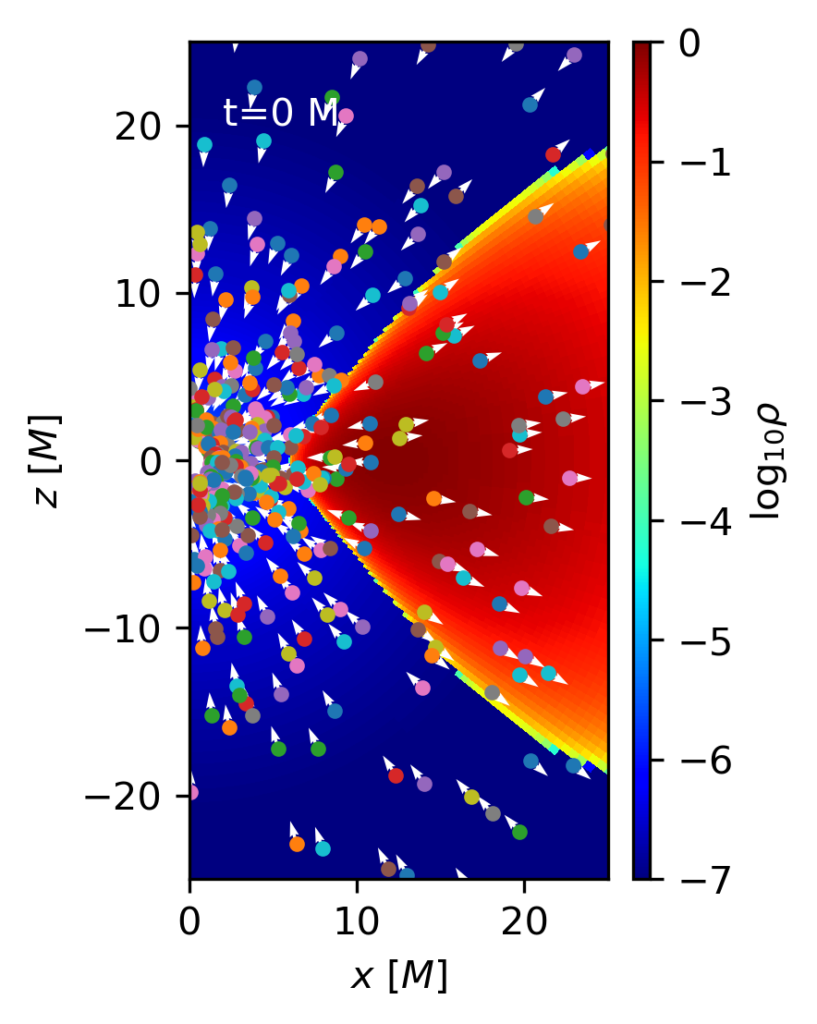
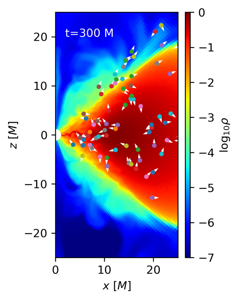
However, although plotting these arrows is useful as an example, it is important to mention that these are not the coordinate velocity at which particles are moving on the domain, which should include the shift and lapse functions.