First session
I. Installing and running a first simulation with BHAC
Follow the steps in the tutorial “Getting started” at https://bhac.science/documentation/
In case you are using a Windows machine, you probably need to follow the steps here: https://docs.google.com/document/d/1RZxIFZogpx6BDUvSSi8g_oUUhW6AvGpq9fCj7weasFk/edit?usp=sharing
II. Visualizing the output
1. Setting up the BHAC python tools
You may need to install ipython3 and vtk. On a Linux terminal, you can do so by typing
sudo apt install ipython3
sudo apt-get install python3-vtk7
And following the instructions.
Now we need to set-up the path to the BHAC python tools. To do so, open the file .bashrc in your home directory, and add the line
export PYTHONPATH = $BHAC_DIR/tools/python:$PYTHONPATH
Just after the definition of BHAC_DIR.
Back on the terminal, type:
source ~/.bashrc
Now we should be ready to visualize BHAC data using ipython.
2. Plotting data
Inside the directory shockTube, run ipython3 with
ipython3 --pylab
and load the BHAC python tools by typing
import read, amrplot
Now we can load one of the output files from our previous run using
d=read.load(0,file='output/data1D',type='vtu')
The data is now stored on the object “d”, and we can query several quantities by looking at its attributes. For example,
d.time contains the time.
d.rho contains the density array (the rest of variables contained in “d” were displayed at the time of loading it).
We can get the positions and store them in the array x by doing:
x=d.getCenterPoints()
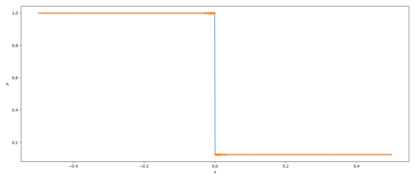
and plot the spatial distribution of density using
plt.plot(x,d.rho)
We can also plot with crosses in order to visualize the different AMR levels.
plt.plot(x,d.rho,'+')
You might notice how the resolution increases close to the discontinuity.
Now we can read the second snapshot, using
e=read.load(1,file='output/data1D',type='vtu')
and repeat the steps. To which time does this snapshot correspond? How does density and other quantities look like? What is the behaviour of mesh refinement?
III. Changing the parameters
- Number of adaptive mesh refinement levels
The number of AMR levels is controlled by the parameter ‘mxnest’ in the parameter file, amrvac1D.par. You may try increasing or decreasing by one the number of levels in the simulation, runnning and plotting again.
- Reconstruction
The type of reconstruction is controlled by the variable ‘typelimiter1’. Set it to ‘minmod’ instead of ‘cada3’. What is the difference in sharpness between the solution obtained with minmod and that obtained with cada3? For the complete list of reconstruction techniques available in BHAC, you can have a look at the manual at https://bhac.science/documentation_html/par.html and look for ‘typelimiter1’.
- What else can you change?
Primera sesión
I. Instalación de BHAC y primera simulación
Siga los pasos en el tutorial“Guía de iniciación” en https://bhac.science/documentation/
En caso de que esté utilizando una máquina con Windows, probablemente deba seguir los pasos descritos aquí: https://docs.google.com/document/d/1RZxIFZogpx6BDUvSSi8g_oUUhW6AvGpq9fCj7weasFk/edit?usp=sharing
II. Visualización de los datos
1. Configuración de las herramientas de Python de BHAC
Es posible que deba instalar ipython3 y vtk. En una terminal de Linux, puede hacerlo escribiendo
sudo apt install ipython3
sudo apt-get install python3-vtk7
Y siguiendo las instrucciones.
Ahora necesitamos configurar la ruta a las herramientas de Python de BHAC. Para hacerlo, abra el archivo .bashrc en su directorio personal y agregue la línea
export PYTHONPATH = $ BHAC_DIR / tools / python: $ PYTHONPATH
Justo después de la definición de BHAC_DIR.
De vuelta en la terminal, escriba:
source ~ / .bashrc
Ahora deberíamos estar listos para visualizar los datos de BHAC usando ipython.
2. Graficando
Dentro del directorio shockTube, ejecute ipython3 con
ipython3 --pylab
ó
ipython --pylab
y cargue las herramientas de Python BHAC escribiendo
import read, amrplot
Ahora podemos cargar uno de los archivos de salida de nuestra primera simulación usando
d=read.load(0,file='output/data1D', type = 'vtu')
Los datos ahora se almacenan en el objeto “d”, y podemos consultar varias cantidades observando sus atributos. Por ejemplo,
d.time contiene el tiempo.
d.rho contiene el arreglo de la densidad (el resto de variables contenidas en “d” se muestran al momento de cargar el archivo).
Podemos obtener las posiciones y almacenarlas en el arreglo ‘x’ haciendo:
x=d.getCenterPoints()
y graficar la distribución espacial de la densidad usando
plt.plot(x,d.rho)
También podemos graficar con cruces para visualizar los diferentes niveles de AMR.
plt.plot(x,d.rho,'+')
Observe cómo la resolución aumenta cerca de la discontinuidad.

Ahora podemos leer el siguiente archivo, usando
e=read.load(1,file='output/data1D', type='vtu')
y repetir los pasos. ¿A qué tiempo corresponde este archivo? ¿Cómo se ven la densidad y otras cantidades? ¿Cuál es el comportamiento del refinamiento de la malla?
III. Cambiando otros parámetros
- Número de niveles de refinamiento de malla adaptativa
El número de niveles de AMR se controla mediante el parámetro ‘mxnest’ en el archivo de parámetros, amrvac1D.par. Puede intentar aumentar o disminuir en uno el número de niveles de la simulación, correr de nuevo y volver a graficar.
- Reconstrucción
El tipo de reconstrucción está controlado por la variable ‘typelimiter1’. Configúrelo en ‘minmod’ en lugar de ‘cada3’. ¿Cuál es la diferencia de nitidez entre la solución obtenida con minmod y la obtenida con cada3? Para obtener la lista completa de técnicas de reconstrucción disponibles en BHAC, puede consultar el manual en https://bhac.science/documentation_html/par.html y buscar ‘typelimiter1’.
- ¿Qué otros parámetros se pueden cambiar?