I. Turbulent accretion disk simulation
Go to the ‘bhac_runs’ directory that you created in the first session and copy the ‘FMTorus’ test from the BHAC files in the same way as you did with the tests in the previous tutorials.
Inside the new FMTorus directory, use the configuration line
$BHAC_DIR/setup.pl -d=23 -phi=3 -z=2 -g=24,16 -p=rmhd -eos=gamma -nf=1 -arch=gfortran -coord=mks
and compile the test with
make
To have a set-up that we can run within a reasonable time, we must reduce the resolution. In the parameter file amrvac.par, set the number of AMR levels to 1 and the resolution to 48×24 with
mxnest = 1
nxlone1 = 48
nxlone2 = 24
We want the set-up to run until t = 500, so in the &stoplist we comment the completion condition based on iterations (itmax) and set the one based on time (tmax) to 500
! itmax = 1000
tmax = 500
To avoid generating many files and filling up our hard drive, we reduce the frequency of the output by setting the following &savelist parameters in these values
ditsave (1) = 10
dtsave (2) = 10
dtsave (5) = 0.1
The total output should not exceed 2GB. Finally, specify the output to a directory whose name refers to the number of AMR levels used, setting
filenameini = 'outputAMR1/data'
filenameout = 'outputAMR1/data'
filenamelog = 'outputAMR1/amrvac'
Once you finished editing the parameter file, make sure to create that directory
mkdir outputAMR1
As the simulation can progress slowly, we free the terminal and redirect the output running with
mpiexec -n N ./bhac &> outputAMR1/out &
With N the number of CPUs that we want to use (this test can be executed in a maximum of 9 CPUs). We can monitor the status of the simulation with
tail -f outputAMR1/out outputAMR1/amrvac.log
The last column shows the expected time to finish the simulation in hours, while the first shows the number of iterations and the second the elapsed time in simulation units.
Ib. Restarting a simulation from a file
Many times we must interrupt a simulation before the time we want to reach (for example, if we need to turn off the computer).
We can restart a simulation from, e.g., the data0075.dat file, running with
mpiexec -n N ./bhac -restart 75
The root of the file name must be specified in the parameter file, by the filenameini parameter.
II. Analysis
As in the previous sessions, we can visualize a snapshot of the simulation with ipython, loading the BHAC tools read and amrplot and reading one of our output files
d = read.load(iFile,file='output/data',type='vtu')
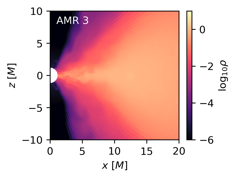
where iFile is the index of the file, and plotting, for example, the density
p1=amrplot.polyplot(np.log10(d.rho),d,xrange=[0,50],yrange=[- 50,50])
The plot should show a torus that becomes more and more turbulent until it begins to feed the black hole at the origin.
However, in addition to visualizing the 2D distribution, this test contains other diagnostic tools. For example, we can visualize different time series by reading the file data_analysis.t
Fluxes=np.loadtxt('outputAMR1/data_analysis.csv')
The first column contains the time, and the second the accretion rate of the black hole measured at the horizon . We can visualize it by closing the window of the previous visualization and typing
t=Fluxes[:,0]
mdot=Fluxes [:,1]
plt.plot(t,mdot)
III. Increasing the resolution.
Run new simulations increasing the resolution in the areas of interest by adding more levels of AMR, that is, changing the mxnest parameter to 2, 3 and 4. Do not forget to also modify the parameters that specify the input and output directories filenameini, filenameout, filenamelog and to create the directories outputAMR2, outputAMR3, and outputAMR4.
Using a single CPU, each simulation should be completed in about these times:
AMR1: 2 minutes
AMR2: 20 minutes
AMR3: 1.5 hours
AMR4: 9 hours
Once all simulations are completed, we can compare their accretion rates.
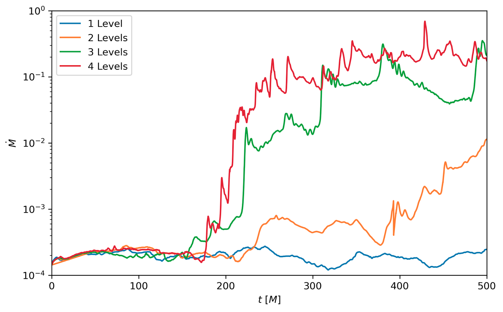
You may notice that when increasing the resolution, accretion starts closer to a value around t=200 M; that is, we have a global property that converges with the resolution. Once accretion starts, it also acquires it also gets closer to a similar value when increasing resolution.
If we visually compare the final state of the simulations, we also see that some features change with increasing resolution. For example, very low-resolution simulations show a high-density mini-torus, due to the fact that matter accumulates there as it cannot lose angular momentum because the magneto-rotational instability is not sufficiently resolved.


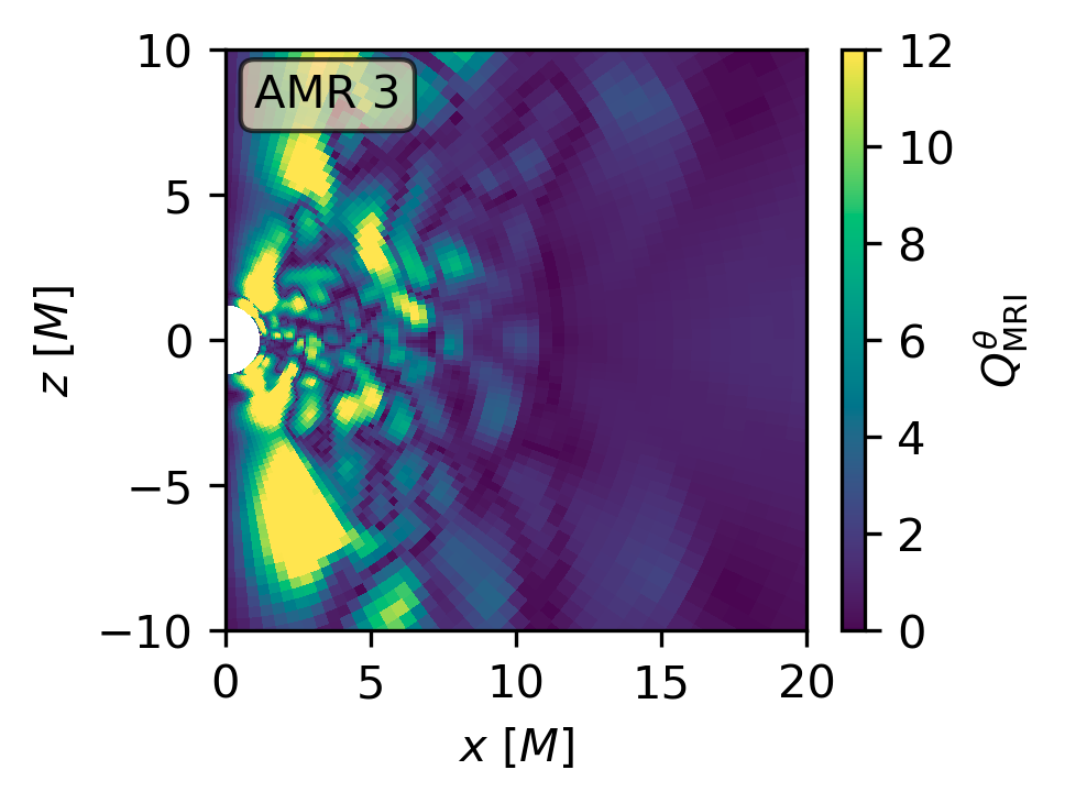
Finally, in this test it is also possible to plot the MRI quality factor (d.Qr, d.Qtheta, d.Qphi). The minimum value recommended by Sano et al. (2004) to achieve a correct saturation of the MRI is 6.


Sesión 3
I. Simulación de disco de acreción turbulento
Sitúese en el directorio ‘bhac_runs’ que creó en la primera sesión y copie el test ‘FMTorus’ de los archivos de BHAC del mismo modo que hizo con los tests de los tutoriales anteriores.
Dentro del nuevo directorio FMTorus, use la línea de configuración
$BHAC_DIR/setup.pl -d=23 -phi=3 -z=2 -g=24,16 -p=rmhd -eos=gamma -nf=1 -arch=gfortran -coord=mks
y compile el test con
make
Para tener un set-up que podamos correr dentro de un tiempo razonable, debemos reducir la resolución. En el archivo de parámetros amrvac.par, fije el número de niveles AMR a 1 y la resolución a 48×24 con
mxnest = 1
nxlone1 = 48
nxlone2 = 24
Buscamos que el set-up corra hasta el t=500, por lo que en la &stoplist comentamos la condición de finalización basada en las iteraciones (itmax) y fijamos la basada en el tiempo (tmax) en 500
!itmax = 1000
tmax = 500
Para evitar generar muchos archivos y llenar nuestro disco duro, reducimos la frecuencia de la salida fijando los siguientes parámetros de la &savelist en estos valores
ditsave(1) = 10
dtsave(2) = 10
dtsave(5) = 0.1
El total de archivos generados en este tutorial no debería exceder los 2GB. Finalmente, especifique la salida hacia un directorio cuyo nombre haga referencia al número de niveles AMR usados, fijando
filenameini = 'outputAMR1/data'
filenameout = 'outputAMR1/data'
filenamelog = 'outputAMR1/amrvac'
Una vez editado el archivo de parámetros, asegúrese de crear ese directorio
mkdir outputAMR1
Como la simulación puede avanzar lentamente, al iniciarla liberamos la terminal y redirigimos el output usando
mpiexec -n N ./bhac &> outputAMR1/out &
Con N el número de CPUs que deseamos usar (este test puede ejecutarse máximo en 9 CPUs). Podemos monitorear el estado de la simulación con
tail -f outputAMR1/out outputAMR1/amrvac.log
La última columna muestra el tiempo esperado para finalizar la simulación en horas, mientras que la primera muestra el número de iteraciones y la segunda el tiempo transcurrido en unidades de tiempo de la simulación.
Ib. Continuar una simulación a partir de un archivo
Muchas veces debemos interrumpir una simulación antes del tiempo al que deseamos llegar (por ejemplo, tenemos que apagar la computadora).
Podemos reiniciar una simulación a partir del archivo data0075.dat usando por ejemplo
mpiexec -n N ./bhac -restart 75
La raíz del nombre del archivo debe estar especificada en el archivo de parámetros, por el parámetro filenameini.
II. Análisis
Igual que en la sesiones anteriores, podemos visualizar una instantánea de la simulación con ipython, cargando las herramientas de BHAC ‘read’ y ‘amrplot’ y leyendo uno de nuestros archivos de salida
d=read.load(iFile,file='output/data', type = 'vtu')
donde iFile es el índice del archivo, y graficando, por ejemplo, la densidad
p1=amrplot.polyplot(np.log10(d.rho),d,xrange=[0,50],yrange=[-50,50])
La gráfica debería mostrar un toroide que se va haciendo cada vez más turbulento hasta que comienza a alimentar el agujero negro situado en el origen.
Sin embargo, además de visualizar la distribución 2D, éste test contiene otras herramientas de diagnóstico. Por ejemplo, podemos visualizar distintas series de tiempo leyendo el archivo data_analysis.t
Fluxes=np.loadtxt('outputAMR1/data_analysis.csv')
La primera columna contiene el tiempo, y la segunda la tasa de acreción del agujero negro medida en el horizonte. La podemos visualizar cerrando la ventana de la visualización anterior y tecleando
t=Fluxes[:,0]
mdot=Fluxes[:,1]
plt.plot(t,mdot)
III. Aumentando la resolución.
Ejecute nuevas simulaciones aumentando la resolución en las zonas de interés agregando más niveles de AMR, es decir, cambiando el parámetro mxnest a 2, 3 y 4. No olvide modificar también los parámetros que especifican los directorios de entrada y salida filenameini, filenameout, filenamelog y crear los directorios outputAMR2, outputAMR3 y outputAMR4.
Usando un único CPU, cada simulación se completaría aproximadamente en este tiempo:
AMR1: 2 minutos
AMR2: 20 minutos
AMR3: 1.5 horas
AMR4: 9 horas
Una vez que todas las simulaciones hayan concluido, podemos comparar las tasa de acreción

Se puede notar que al aumentar la resolución la acreción inicia cada vez más cerca de un valor al rededor de t=200; es decir, tenemos una propiedad global que converge con la resolución. Una vez que la acreción inicia, ésta también adquiere un valor más cercano entre las dos simulaciones de más alta resolución.
Si comparamos visualmente el estado final de las simulaciones, también vemos que algunas características cambian al aumentar la resolución. Por ejemplo, las simulaciones a muy baja resolución muestran un mini-toro de alta densidad, debido a que la materia se acumula allí al no poder perder momento angular ya que la inestabilidad magnetorotacional no está suficientemente resuelta.


En el test es posible graficar el factor de calidad de la MRI (d.Qr, d.Qtheta, d.Qphi). El valor mínimo recomendado por Sano et al. (2004) para alcanzar una correcta saturación de la MRI es 6.


